
Since we saw the fact that the Hough PR actually works with the simplified geometry, it is natural to do the generalization of the Hough PR to the real geometry as my next step. Generation of new Hough Tables is quite easy task. But the design of new PR algorithm was not an easy task mainly because of missing layers. To best deal with the missing layers, we have to consider the match-sticks which jump over a missing layer.
Fortunately, we don't have any two consecutive missing layers. So for a given hit on a layer "i", we can always make a Hough match-stick from the layer to the next consecutive layer, "i+1", or to the next next layer "i+2".
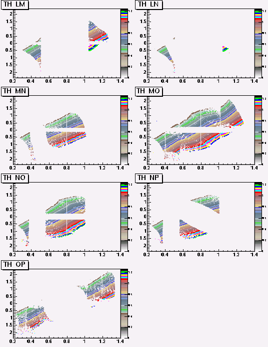
With the simplied geometry, we had 4 combinations of layers, IJ, JK, KM, MO. Now we have 13 combinations, IJ, IK, JK,JL,KL,KM,LM,LN,MN,MO,NO,NP,OP.
Here are the tables.....


Measurement of Errors of Hough Table
Hough transformation means getting momentum and theta infomation from geometrical configuration of two associated hits or match stick. In other words, for a given match stick, we immediately obtain "P" and "theta". A question is naturally arised. With what precision? How much we can rely on the information. Since the Hough Tables are made by the ideal track trajectory (MULS=0 no multiple scattering, LOSS=4 average energy loss), for the realistic case, we must take the measurement error into account.
The simpliest way is making the same binned Hough tables and filling with the measured error and use them together with the Hough table. Let's call it Hough Error Table. A problem is that we need a huge amount of CPU time to have enough statistics for all bins. Since bin to bin fluctuation of errors should not be big (I hope), one may use less coarse bin tables. The stratergy to get the Hough Error Table is
i) Generate N identical particles for a given theta and a momentum with MULS=1, LOSS=3, and fill the variation of 1/P or theta to the fine binning Hough Table(200x400).
ii) Do i) for the full range of theta(25-70 degree) with bigger step (2 degree), and for the full range of momentum (100MeV to 1GeV) with bigger step (10% error)
iii) make a coarse bin Hough Table(20x40). Calculate the average variation over 100 measurement in the fine bin table and fill to the coarse bin table.
The tables have the measured error of Hough components, ie, sigma(1/P),sigma(theta).

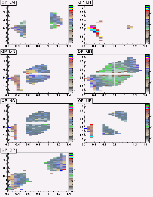
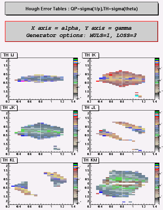
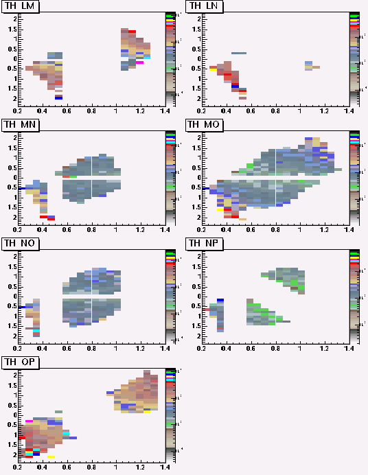
The size of Hough Tables
From now on I will simply call Hough Tables as the set of tables of 1/p, sigma(1/p), theta, sigma(theta). A Hough table for 1/p and theta uses a little bit less than 1 Mbytes (after the compression as it is the default feature of ROOT). Another table uses a half MegaBytes if I use fine bin table(200x400), but this can be reduced hugely by using of real coarse bin table (20x40). In total, I think I will need 1Mbyte for a set of hough table. Considering the z-vertex dependency, from +10cm to -15cm, with a step or variable steps of about half centimeter(if we demonstrate succesfully the interpolation works fine), we will need 50 sets of Hough tables, ie. 50Mbytes, which is not a big value....
Track Reconstruction
In the simplified version, a track consists of 4 match sticks with a
seed, i.e., track seed + IJ + JK + KM + MO.
With our complicated geometry, one should be flexible for the missing
layers. Track finding algorithm now starts from the layer "I" and
try to find match-sticks with the hits on layer "J" which are consistent
with a track seed in theta. If no match stick exists with "J", it tries
with "K".
Then go to the layer "J", and do the same job. I.e., find match sticks with "K" if failed, with "L".
Finally a track candidates means a set of match sticks up to layer "O" or up to layer "P" + a seed.
With this algorithm, a track candidate has no two consecutive missing hits in layers by definition. According to our definition of the"findable" this is good feature!
I remind you the definition.
* Definition of "findable" track
No more than one missing hit in layers A-D
No more than one missing hit in layers E-J
No more than one missing hit in layers K-P
No two consecutive missing hits along the track.
------------------------------
I.e. it's not OK to miss plane D and then also plane E.
NOTE: If the track goes through a region where a layer just doesn't exist, that is not a missing hit, it's a design "feature". If the track goes "outside" the detector in a given layer, that IS a missing hit.
I will apply the findable condition later (not now because it is not urgent matter).
Cuts for the minimization of CPU time and the optimized cut values.
With the track finding algorithm and the Hough tables, the actual CPU time to generated all the track candidates is a little less than INFINITY! This is because we allow all the stupid combination of match sticks, and we consider all the hits even the hits are inconsistent with a given track seed in phi and theta and charge, etc.... Here I summarize all the cuts I invent to minimize the CPU time....
To do this job, I generated 8 different single track event samples. Each sample has 100 events.
200MeV pion+ @theta=28
300MeV pion+ @theta=38
400MeV pion+ @theta=44
500MeV pion+ @theta=45
500MeV pion- @theta=45
400MeV pion- @theta=46
300MeV pion- @theta=52
200MeV pion- @theta=62
These samples are chosen very carefully in order to explore all the difference spectrometer regions.
And I generated 100 events having the above 8 tracks per event, and a typical Au-Au interaction for final test.
Again the cone size for the track seed finding is 0.02 in eta-phi space.
For a given track seed,
Cut 1 (vertical hit position)
Extrapolate the track to a layer, and calculate "y" position (y_seed). Compare the difference between y_hit and y_seed with its error, where the error is assumed a quadrature sum of PadSizeY/sqrt(12) and input Phi error.
| y_hit - y_seed | > sqrt( PhiError^2 + PadSizeY^2/12)
Here is the efficiency versus PhiError for 200MeV pion+.
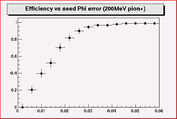
0.03 looks like stringent, 0.05 is look like very conservative.
Cut 2 (charge correlation of hit horizontal position and the track seed direction)
Given the setup magnetic field, a positive track bends toward to the beam pipe. So the outer layer hits have smaller polar angles (theta) than those of the straight line part hits. For a negative track, this is reverse. Reconstruction is done by two steps according to the charge. So when we reconstruct the positive charged tracks, we need to consider only hits having smaller theta value than that of the given track seed. This is clear if you see the following picture.

The plot shows the distribution of "theta_layer_I "- "theta_seed" for the 8-track event sample. As one can see the charge correlation is clear.
(theta_layer - theta_seed)*charge
> 0
Cut 3 (maximum allowed theta difference for hits on layer I)
As shown in the above plot, most of hits are in the range of +-0.04 because of the smallness of magnetic field up to the layer I. When generates the track candidate we only consider hits within the range.
|theta_layer_I - theta_seed|< 0.04
This cut is only to reduce the CPU time. One can do the same for the layer J, etc..
Cut 4 (Match-stick theta value should be consistent with the track seed)
After the cleaning of hits by Cut1 and Cut2, Hough match-sticks are formed by hits from layer "i" with "i+1", or with "i+2". Match sticks are rejected if theta value is not consistent with the track seed.
|theta_ms - theta_seed|>sqrt(sigma_theta_seed^2+sigma_theta_ms^2)

Where sigma_theta_ms is the measured value and sigma_theta_seed is optimized value after looking the above plot. sigma_theta_seed is set to 0.02.
Cut 5 (When chaining Match sticks, variation of theta value should be small)
When create the track candidates, i.e., chaining Match sticks, we should allow chaining them only when the variation of theta is small.
|theta_ms_i - theta_ms_j| > N x sqrt(sigma_theta_i^2 + sigma_theta_j^2)
where N is set to 2.

1.5 sigma looks like O.K.
Cut 6 (Momentum variation should be small)
The same cut as the Cut 5, but for momentum measurement.
| (1/P)_i - (1/P)_j | > N x sqrt(
sigma_1/p_i ^2 + sigma_1/p_j^2)
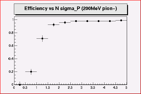
2.5 sigma looks o.k.
Cut 7 (cuts not necessarily needed, but help to reduce the number of candidates about 10%)
There must exist at least 3 hits in layers E,F,G,H between theta_s
and theta_layer_I. This is almost true except for the case of bad multiple
scattering.
After all these cuts, I run the algorithm for a realistic Au-Au
event. I have the following picture.
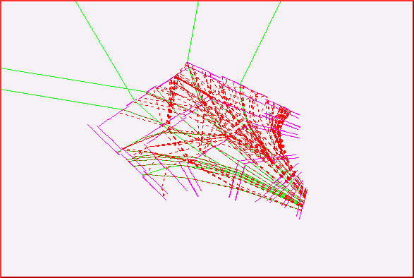
There are 16 findables with the follwoing findable definition which is a little bit different from the one decided in the meeting in February.
For layers AB,CD : at least 3 hits (i.e. one missing hit)
For layers EF,GH,IJ : at least 4 hits (1 hit can be lost due to a missing
layer on G or H, and a real missing hit, so allow two missing hits )
For layer KL, MN, OP: at least 3 hits ( for central region , there
are 4 layers only, allowing one missing hit)
and there is no two successive missing hits for two consecutive layers.
Here are the MC finable list:
Event 0 has 16171 MC tracks and 17440 MC hits
Q P
theta phi
#hit #merged hits # hits per layer
findable 0:
-1 0.285 51.967 -0.023
14 13 1111111011101021
findable 1:
-1 0.160 48.826 -0.013
14 13 1112111011011011
findable 2:
-1 0.848 44.553 0.015
17 13 3211111110101120
findable 3:
-1 0.179 30.837 -0.024
20 14 1211110131102212
findable 4:
1 0.596 41.368 0.029
15 14 1112111111101101
findable 5:
-1 0.775 28.608 -0.035
13 13 1111110111101110
findable 6:
-1 0.262 54.139 0.050
16 14 1111211011111012
findable 7:
-1 0.662 34.956 -0.019
18 13 3211110112101120
findable 8:
1 0.527 43.224 -0.007 21
15 3111111121202112
findable 9:
1 0.820 48.220 0.033
16 13 2111111022101110
findable 10:
1 0.896 53.732 0.019
16 13 1121121021101110
findable 11: -1
0.422 53.090 0.022 14
12 1111111011201020
findable 12:
1 0.363 33.260 -0.008 18
14 2111210111111022
findable 13: -1
0.246 48.959 0.045 15
12 1111211012201010
findable 14: -1
0.266 50.392 -0.043 14
13 1111111011101021
findable 15: -1
0.377 62.825 0.049 16
14 1211111012111011
Number of MC seeds &
findables: 32 16
And I have 41 reconstructed seeds, and 461 track candidates.
Now a big question is that whether we have correctly reconstructed the MC findables or not, in other words, whether we keep them in our 461 candidates, or we just created 461 ghosts.....
So I made a simple minded routine which select the best mactching candidates to the MC findables. & reconstructed ones. For a given track seed, I first find a MC findable which is closest to the seed in theta phi space. Then for this MC findables, I found a reconstructed track candidates which share maximally the hits.
After the selection (let's say the selection by MC truth information.
Or theoretically the best selection algorithm).
I have this.

So I reconstructed 14 good tracks, and 2 lost, no ghost (by my eyes again). This means the efficiency of the algorithm is 0.875 and no ghost... This numbers are important because these are the best value we can obtain (because we are using perfect selection algorithm).
Next step
My next step is of cause finding a good algorithm to select maximally
the MC findables. We may have to rely on chi2 cut from track fitting
and/or particle id information. I am planning to use both. We may be able
to use just our pregenerated Templates for this (Themplates will let us
know "p" and chi2 too). But I am worrying about CPU time then.... Let's
discuss on Monday.