LQSGW
LQSGW: Ab initio electronic structure code
Our parallel ab initio electronic structure code, LQSGW, lies at the heart of Comsuite, as it is a basic building block for the theoretical calculation of material properties. Calculation of electronic structure can be understood mathematically as an eigenvalue problem in which the determination of the electron self¬-energy matrix Σ is the main challenge. LQSGW offers several levels of approximations to Σ: DFT, Hartree-Fock, self-consistent GW, and linearized quasiparticle GW. These approaches allow one to study the electronic structure, i.e. the ground state and excited state electronic properties, of weakly to moderately correlated materials. One can study strongly correlated materials by using ComDMFT or ComRISB, which combine LQSGW with DMFT and with the Gutzwiller approximation.
MPI Parallelization
LQSGW uses MPI for its parallelization. It generally uses two-dimensional schemes for parallelization based on momentum, and time or frequency. It is possible to configure the parallelization, controlling the partitioning along each of the two dimensions. LQSGW can scale successfully to a thousand or more processors.
Limitations
GW is limited to calculating only certain diagrams contributing to the electronic self-energy; therefore it is limited to materials which are not too strongly correlated. For strongly correlated materials it is more appropriate to ComDMFT or ComRISB, which combine LQSGW with DMFT or with the Gutzwiller approximation.
LQSGW implements non-relativistic, scalar-relativistic (2 component), and fully-relativistic (4 component) calculations. Every calculation done with LQSGW includes both muffin-tin regions around each atom, and also an interstitial region in the volume not occupied by muffin tins. LQSGW's DFT calculations allow fully relativistic calculation of both the muffin tins and the interstitial region. However, for all methods beyond DFT LQSGW is limited: it does not allow fully-relativistic (4 component) calculations of the interstitial region. If the user specifies a 4 component calculation, then the muffin-tin region is done with the 4 component formalism and the interstitial region is done with the 2 component formalism. This limitation does not apply to DFT calculations.
For all methods beyond DFT, LQSGW performs its calculations seamlessly in imaginary time and imaginary frequency. Results on the axis of real frequency (energy) can be obtained only by analytical continuation.
Appendix A: Selecting the muffin tin radii
A critical aspect of the LAPW basis is that the model of atomic basis functions within the muffin tin radius joining to plane waves in the interstitial region, does not allow for overlapping muffin tin radii. As a starting point predefined radii are used that are stored within the input generator. In practice these radii might violate the no-overlap requirement as different crystal structures may have very different atom packing. Therefore we consider all different atom pairs and test for each pair whether the sum of initial muffin tin radii exceeds the minimal distance between the atoms. If the sum of the radii is greater than the inter-atom distance then a smaller muffin tin radius is calculated as
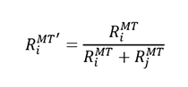
For a given atom i the smallest value of RiMT' is selected as the final muffin tin radius.
Initial muffin tin radii for the elements of the periodic table based on Elk 3.1.12.
| Elements | Initial Radius |
|---|---|
| H - He | 1.4 |
| Li - O | 1.8 |
| F | 2.0 |
| Ne | 1.6 |
| Na - Cl | 2.2 |
| Ar | 2.0 |
| K - Br | 2.4 |
| Kr | 2.2 |
| Rb - I | 2.6 |
| Xe | 2.4 |
| Cs - At | 2.8 |
| Rn | 2.6 |
| Fr - Ts | 3.0 |
| Og | 2.8 |
The initial values for the radii are given in Initial muffin tin radii for the elements of the periodic table based on Elk 3.1.12.
Appendix B: Choosing the basis set
LQSGW uses the LAPW basis. This basis consists of two parts:
- Atomic wave functions within a muffin tin radius
- Plane waves in the interstitial region
The atomic to plane wave matching condition
In order for the orbitals to be defined properly they have to continuous at the muffin tin radius, and for the kinetic energy to be well defined they also have to have a continuous first order derivative at that radius. In practice that means that the atomic and the plane wave basis functions cannot be selected independently. Instead, they have to chosen such that the continuity equations have a solution. In addition the plane wave basis set has to be chosen in accordance to the cutoff energy. In practice the continuity conditions along with the chemical element dependent highest occupied orbital angular momentum determine a lower limit on the plane wave cutoff. As this is a minor issue that aspect will not be discussed here.
In his book Singh [Singh 1994] showed that in order for the plane waves to match the oscillations of the spherical harmonics of the atomic basis functions the condition
RMT K = lmax
must hold. Here RMT is the muffin tin radius for a particular element, lmax is the maximum angular momentum basis function on that element, and K is the plane wave cutoff. Hence once the cutoff energy is specified and the muffin tin radii are established the maximum angular momentum for each element can be calculated. The atomic basis set is then composed from stored data, automatically extended up to the required maximum angular momentum.
The impact of the packing factor
An additional complication stems from different basis set requirements depending on the packing factor of a material. For close packed materials the packing factor is high (around 0.74) and the interstitial region is small. Materials such as, for example diamond, have a small packing factor (around 0.34) and correspondingly the interstitial region is large. For the latter kind of materials the quality of the basis set depends more strongly on the number of plane waves. Hence a linear relation is used to scale the plane wave basis set up by a factor 1 to 2 when the packing factor goes down from 0.5 to 0.3.
The choice of atomic basis functions
The atomic basis functions within the muffin tin radius have to chosen with a few considerations in mind:
- Inner core orbitals are compact and not affected by their environment
- Core orbitals are relatively compact and therefore local
- Valence orbitals are key to the interaction of atoms with their environment
- Virtual orbitals do not directly impact the physical properties
These considerations motivate a number of choices. One general choice stems from the fact that the occupied orbitals are clearly defined by the Schrodinger equation. By this we mean that any changes to these orbitals directly impact the physical properties of the system, in particular the total energy. Therefore the linearization energies can be determined safely from solving the atomic Schrodinger equation. The virtual orbitals do not directly affect the physical properties. They only affect these properties in as much as they mix with the occupied states. Hence optimizing their linearization energies based on the Schrodinger equation is risky. Therefore it is preferable to freeze their linearization energies at their initial values. In addition to these general considerations the above conditions lead to the following choices:
The inner core orbitals are solved from the atomic Schrodinger equation. The linearization energies are updated throughout the calculation. Once the DFT phase of the calculation is completed the Hartree-Fock equations are used to solve for the inner core orbitals.
The core orbitals are chosen to be local within the muffin tin radius (i.e., they are guaranteed to go to zero at the muffin tin radius and are therefore marked as “LOC”). This also means that they are not matched to the interstitial wavefunctions that are expressed in plane waves. Their linearization energy is given an initial value that is further optimized throughout the initial DFT calculation.
The valence orbitals will spill out of the muffin tin sphere, and are therefore matched to the interstitial orbitals. In particular the valence s-, and p-orbitals are marked at “APW”. The valence f-orbitals by contrast are so compact that they are local, marked as “LOC”. The valence d-orbitals are somewhere in between. Typically the highest occupied orbital is marked as “APW”. Again their linearization energies are well defined by the Schrodinger equation and hence they can be optimized throughout the DFT calculation.
The virtual orbitals are less well defined the atomic Schrodinger equation. They contribute mainly by mixing with the occupied states. Hence they are considered to be local (marked as “LOC”) and forced to go to zero at the muffin tin radius. Their linearization energies are kept fixed at their initial values.
The orbital linearization energies are initialized according to P = N + ½ - arctanD/π , where N is the principal quantum number of the orbital, and D is the logarithmic derivative of the orbital at the muffin tin radius.
The core, valence, and the lowest virtual orbitals are stored in a table in the input generator. Depending on the cutoff energy additional virtual orbitals can be generated and added as needed by a simple algorithm. The valence orbitals are essentially the highest occupied orbitals. Last, core orbitals are the remaining orbitals stored. Because these core orbitals are optimized during the DFT calculation the quality of the results may depend on how deep in energy the transition between core and inner core orbitals is chosen. In particular in the block between Si and Te it was found that extending the core orbitals one s- and p-shell further down was essential to obtain good band structures.